|
The propositional satisfiability problem (often called SAT) is the problem of determining whether a set of sentences in Propositional Logic is satisfiable. The problem is significant both because the question of satisfiability is important in its own right and because many other questions in Propositional Logic can be reduced to that of propositional satisfiability. In practice, many automated reasoning problems in Propositional Logic are first reduced to satisfiability problems and then by using a satisfiability solver. Today, SAT solvers are commonly used in hardware design, software analysis, planning, mathematics, security analysis, and many other areas.
In the chapter, we look at several basic methods for solving SAT problems. We begin with a review of the Truth Table Method. We then introduce the Backtracking Approach, and we show how it can be improved with Simplification and Unit Propagation. We briefly mention the popular DPLL method. Finally, we talk about non-guaranteed methods, with emphasis on one particular method, called GSAT.
Let Δ = {p∨q, p∨¬q, ¬p∨q, ¬p∨¬q∨¬r, ¬p∨r}. We want to determine whether Δ is satisfiable. So, we build a truth table for this case. See below.
| p |
q |
r |
p∨q |
p∨¬q |
¬p∨q |
¬p∨¬q∨¬r |
¬p∨r |
Δ |
| 0 |
0 |
0 |
0 |
1 |
1 |
1 |
0 |
0 |
| 0 |
0 |
1 |
0 |
1 |
1 |
1 |
1 |
0 |
| 0 |
1 |
0 |
1 |
0 |
1 |
1 |
1 |
0 |
| 0 |
1 |
1 |
1 |
0 |
1 |
1 |
1 |
0 |
| 1 |
0 |
0 |
1 |
1 |
0 |
1 |
0 |
0 |
| 1 |
0 |
1 |
1 |
1 |
0 |
1 |
1 |
0 |
| 1 |
1 |
0 |
1 |
1 |
1 |
1 |
0 |
0 |
| 1 |
1 |
1 |
1 |
1 |
1 |
0 |
1 |
0 |
There is one row for each possible truth assignment. For each truth assignment, each of the sentences in Δ is evaluated. If any sentence evaluates to 0, then Δ as a whole is not satisfied by the truth assignment. If a satisfying truth assignment is found, then Δ is determined to be satisfiable. If no satisfying truth assignment is found, then Δ is unsatisfiable. In this example, every row ends with Δ not satisfied. So the truth table method concludes that Δ is unsatisfiable.
The truth table method is complete because every truth assignment is checked. However, the method is impractical for all but very small problem instances. In our example with 3 propositions, there are 23 = 8 rows. For a problem instance with 10 propositions, there are 210 = 1024 rows - still quite small for a modern computer. But as the number of propositions grow, the number of rows quickly overwhelms even the fastest computers. A more efficient method is needed.
Looking at the example in the preceding section, we can observe that, often times, a partial truth assignment is all that is required to determine whether the input Δ is satisfied.
For example, let's consider the partial assignment {p = 1 , q = 0}. Even without the truth value for r, we can see that ¬p∨q evaluates to 0 and therefore Δ is not satisfied. Furthermore, we can conclude that no truth assignment that extends this partial assignment can satisfy Δ because the sentence ¬p∨q would always evaluate to 0 in every extension. So by determining whether the input in satisfied by a partial assignment, we can save the work of checking all extensions of the partial assignment. In this case, we can conclude that neither the truth assignment {p = 1, q = 0, r = 0} nor the assignment {p = 1, q = 0, r = 1} satisfies Δ. The saving is small in this case; but, as the number of propositions increases, there can be many more truth assignments we can eliminate from consideration. Backtracking allows us to realize this saving.
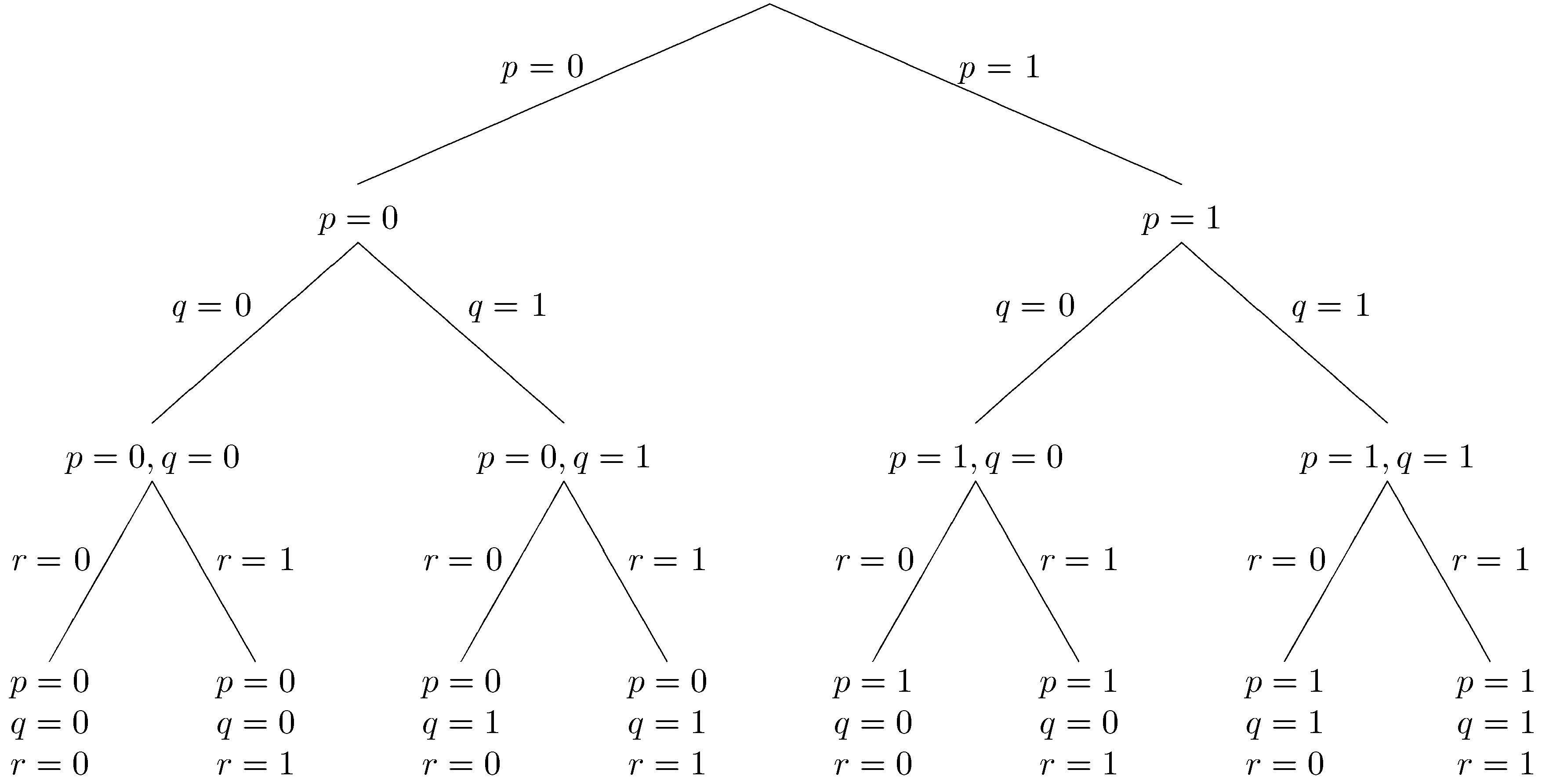
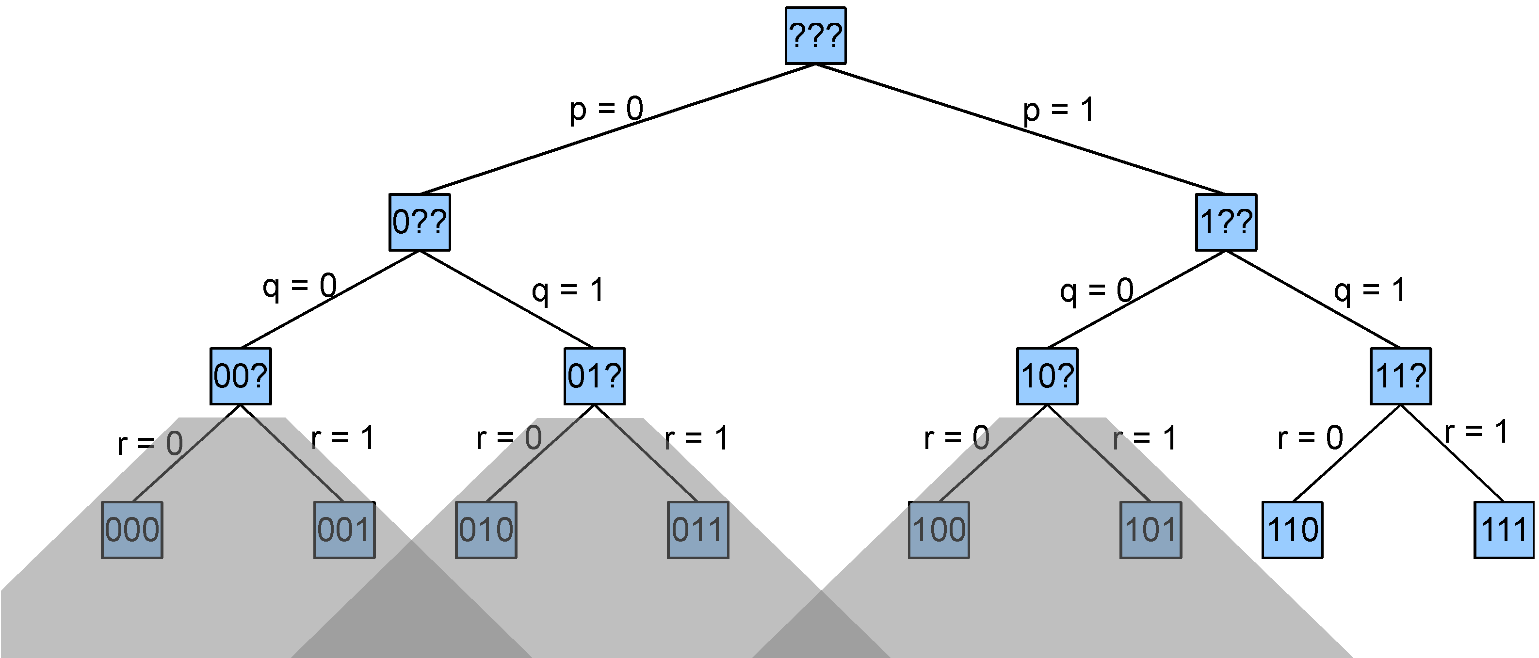
To search the space of truth assignments systematically, both partial and complete, we can set the propositions one at a time. The process can be visualized as a tree search where each branch sets the truth value of a single proposition, each interior node is a partial truth assignment, and each leaf node is a complete truth assignment. Below is a tree whose fringe represents all complete truth assignments.
In basic backtracking search, we start at the root of the tree (the empty assignment where nothing is known) and work our way down a branch. At each node, we check whether the input Δ is satisfied. If Δ is satisfied, we move down the branch by choosing a truth value for a currently unassigned proposition. If Δ is falsified, then, knowing that all the (partial) truth assignments further down the branch also falsify Δ, we backtrack to the most recent decision point and proceed down a different branch. At some point, we will either find a truth assignment that satisfies all the sentences of Δ or determine that none exists.
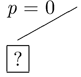
Let's look at an example. At each step, we show the part of the tree explored so far. A boxed node is the current node. An × mark at a node indicates that the truth assignment at that node falsifies at least one sentence in Δ. A ✓ indicates that the truth assignment at that node satisfies all the sentences in Δ. A ? indicates that the partial truth assignment at the node neither satisfies nor falsifies Δ.
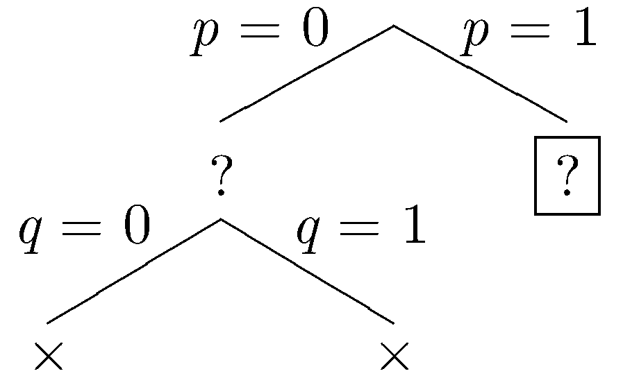
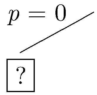
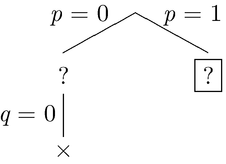
Let's start with the assumption that p is false. This leads to the partial tree shown below.
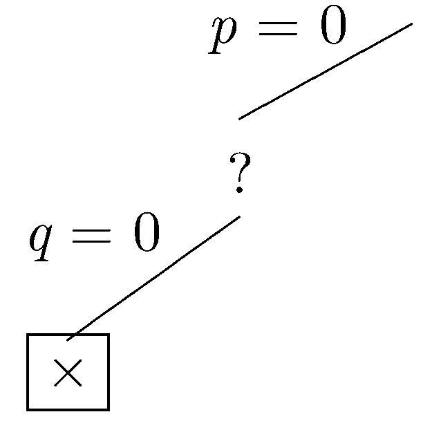
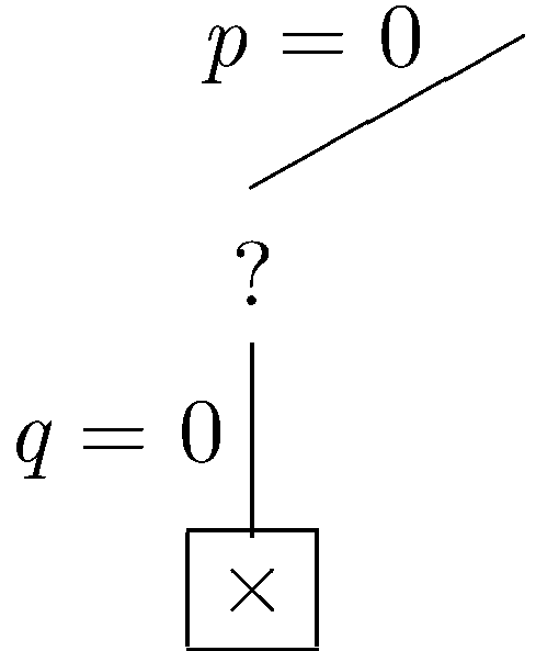
Now, let's assume that q is false. In this case, Δ is falsified, and the current branch is closed.
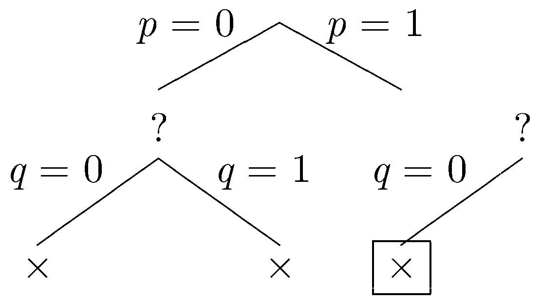
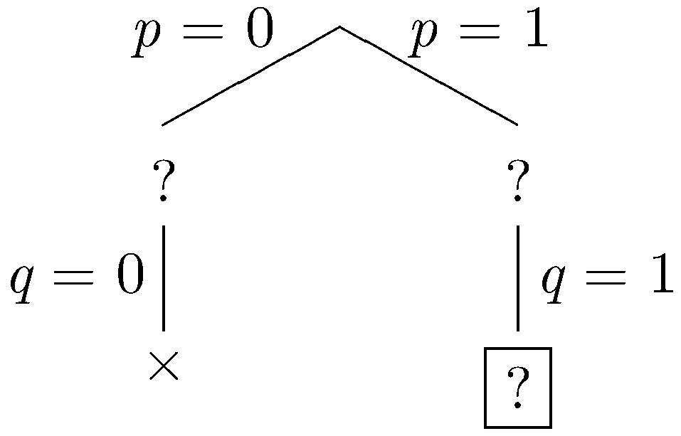
Since the current branch is closed, we backtrack to the most recent choice point where another branch can be taken. This time, let's assume that q is true.
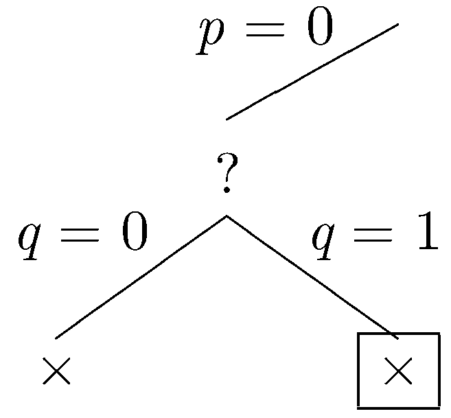
Again, Δ is falsified, and the current branch is closed. Again we backtrack to the most recent choice point where another branch can be taken. Let p be true.
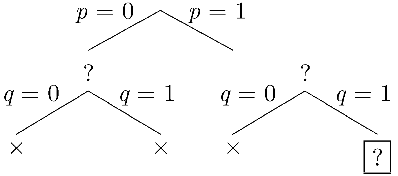
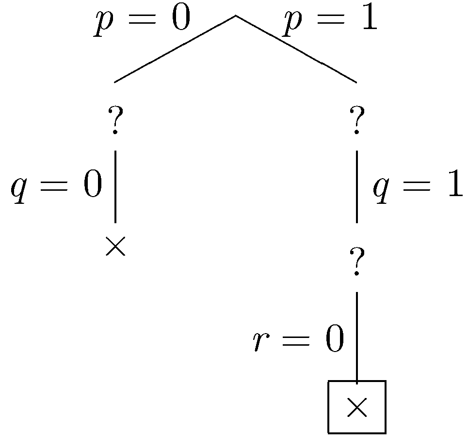
Let q be false.
Again, our sentences are falsified, and we backtrack. Let q be true.
Let r be false.
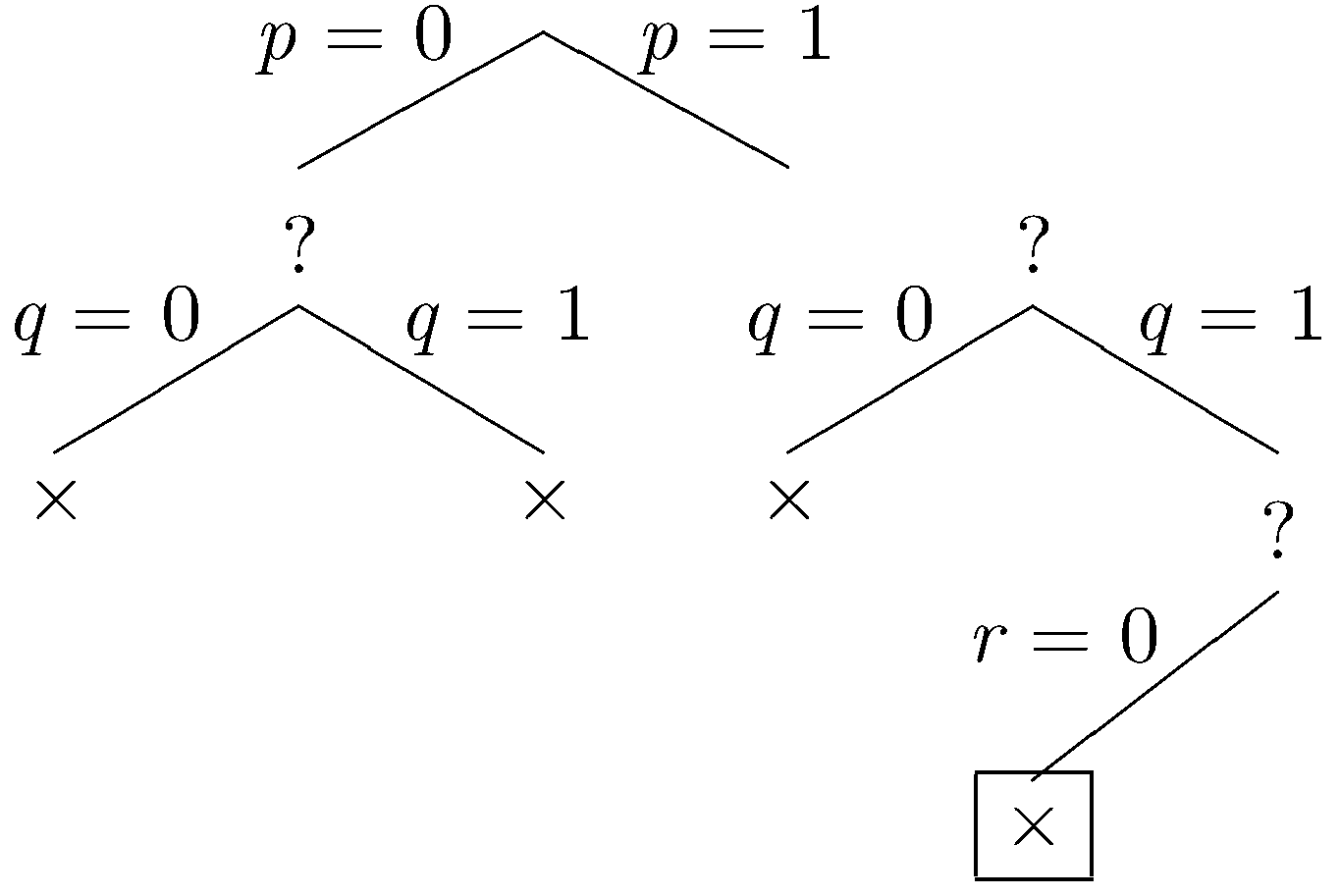
Our sentences are falsified by this assignment, and we backtrack one last time. Let r be true.
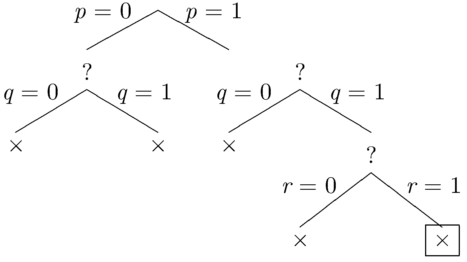
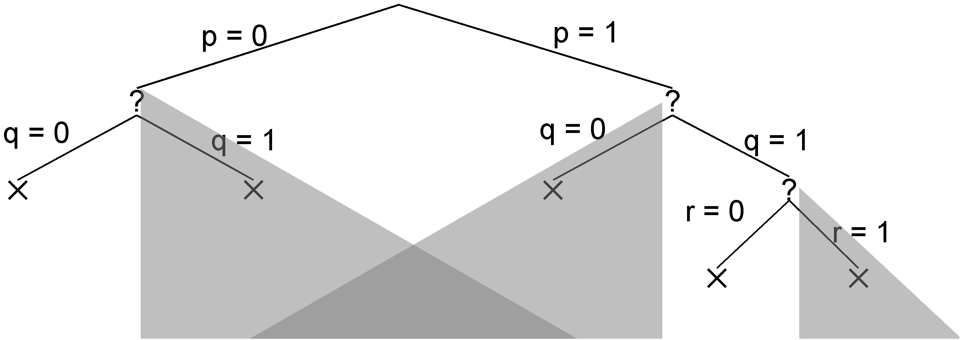
Once again, our sentences are falsified. Since all branches have been explored and closed, the method determines that Δ is unsatisfiable.
Looking at the full search tree compared to the portion explored by the basic backtracking search, we can see that the greyed out subtrees are all pruned from the search space. In this particular example, the savings are not spectacular. But in a bigger example with more propositions, the pruned subtrees can be much bigger.
In this section, we consider two optimizations of basic backtracking search - simplification and unit propagation. In order for these methods to work, we assume that our sentences have been transformed into logically equivalent disjunctions (using a method like the one described in Chapter 5). As we choose the truth values of some propositions in a partial truth assignment for these disjunctions, there are opportunities to simplify the set of sentences that need to be checked.
Suppose, for example, a proposition p has been assigned the truth value 1. (1) Each disjunction containing a disjunct p may be ignored because it must already be satisfied by the current partial assignment. (2) Each disjunction φ containing a disjunct ¬p may be modified (call the result φ') by removing from it all occurrences of the disjunct ¬p because, under all truth assignments where p has truth value 1, φ holds if and only if φ' holds.
If a proposition p has been assigned the truth value 0, we can simplify our sentences analogously. (1) Each disjunction containing a disjunct ¬p may be ignored because it must already be satisfied by the current partial assignment. (2) Each disjunction φ containing a disjunct p may be modified by removing from it all occurrences of the disjunct p.
Consider once again the example in the preceding section. Under the partial assignment p=1, we can simply our sentences as shown below. The first two sentences are dropped, and the literal ¬p is dropped from the other three sentences.
| Original | | Simplified |
|---|
|
| p ∨ q | | − |
| p ∨ ¬q | | − |
| ¬p ∨ q | | q |
| ¬p ∨ ¬q ∨ ¬r | | ¬q ∨ ¬r |
| ¬p ∨ r | | r |
While simplifying sentences is helpful in and of itself, the real value of simplification is that it enables a further optimization that can drastically decrease the search space.
In the course of the backtracking search, if we see a sentence that consists of single atom, say p, we know that the only possible satisfying assignments further down the branch must set p to true. In this case, we can fix p to be true and ignore the subbranch that sets p to false. Similarly, when we encounter a sentence that consists of a single negated atom, say ¬p, we can fix p to be false and ignore the other subbranch. This optimization is called unit propagation because sentences of the form p or ¬p are called units.
Let's redo example 1 with formula simplification and unit propagation. As we proceed through this example, we illustrate each step with the search tree on that step (on the left) and the simplified sentence set (in the table on the right).
To start, let p be false.
 |
|
| Original | | Simplified |
|---|
|
| p ∨ q | | q |
| p ∨ ¬q | | ¬q |
| ¬p ∨ q | | − |
| ¬p ∨ ¬q ∨ ¬r | | − |
| ¬p ∨ r | | − |
|
In the simplified set of sentences, we have the unit ¬q, so we fix q to be false (unit propagation). (We also have the unit q, so we could have fixed q to true. The result is the same in either case.)
 |
|
| Original | | Simplified |
|---|
|
| p ∨ q | | false |
| p ∨ ¬q | | − |
| ¬p ∨ q | | − |
| ¬p ∨ ¬q ∨ ¬r | | − |
| ¬p ∨ r | | − |
|
Δ is falsified, so we backtrack to the most recent decision point, all the way back at the root. Let p be true.
 |
|
| Original | | Simplified |
|---|
|
| p ∨ q | | − |
| p ∨ ¬q | | − |
| ¬p ∨ q | | q |
| ¬p ∨ ¬q ∨ ¬r | | ¬q ∨ ¬r |
| ¬p ∨ r | | r |
|
In the simplified set of sentences, we have the unit q so we do unit propagation, fixing q to be true. (We could also have performed unit propagation using the other unit r.)
 |
|
| Original | | Simplified |
|---|
|
| p ∨ q | | − |
| p ∨ ¬q | | − |
| ¬p ∨ q | | − |
| ¬p ∨ ¬q ∨ ¬r | | ¬r |
| ¬p ∨ r | | r |
|
In the simplified set of sentences, we have the unit ¬r so we do unit propagation, fixing r to be false.
 |
|
| Original | | Simplified |
|---|
|
| p ∨ q | | − |
| p ∨ ¬q | | − |
| ¬p ∨ q | | − |
| ¬p ∨ ¬q ∨ ¬r | | − |
| ¬p ∨ r | | false |
|
Δ is falsified on this branch, so the branch is closed. All branches are closed, so the method determines that Δ is unsatisfiable.
Compared to the tree explored by the basic backtracking search, we see that the greyed out subtrees are pruned away from the search space.
|